Enunţ Teorema creşterilor finite a lui Lagrange mai este deumită şi Prima teoremă a creșterilor finite sau Prima teoremă de medie .
Este o generalizare a teoremei lui Rolle , în care funcția considerată nu are neapărat valori egale la capetele intervalului de definiţie.
Teoremă (Lagrange ).
Fie
f
:
[
a
,
b
]
→
R
,
a
,
b
∈
R
,
a
<
b
{\displaystyle f: [a, b] \rightarrow \mathbb R, \; a, b \in \mathbb R, \; a< b}
funcție care respectă următoarele condiţii:
1) f este continuă pe intervalul închis
[
a
,
b
]
;
{\displaystyle [a, b]; \!}
2) f este derivabilă pe intervalul deschis
(
a
,
b
)
,
{\displaystyle (a, b), \!}
atunci există cel puţin un punct c în intervalul deschis (a, b) (deci
c
∈
(
a
,
b
)
{\displaystyle c \in (a, b) \!}
f
′
(
c
)
=
f
(
b
)
−
f
(
a
)
b
−
a
.
{\displaystyle f'(c) = \frac{f(b) - f(a)}{b-a}. \!}
Consecinţe 1) Dacă f are derivata nulă pe un interval atunci f este constantă pe acel interval.
2) Dacă f , g au derivatele egale pe un interval atunci ele diferă pe acel interval doar printr-o constantă.
f
′
(
x
)
=
g
′
(
x
)
,
∀
x
∈
E
⇒
f
(
x
)
−
g
(
x
)
=
k
,
∀
x
∈
E
.
{\displaystyle f'(x) = g'(x), \; \forall x \in E \; \Rightarrow \; f(x) - g(x) = k, \; \forall x \in E. \!}
3) Dacă derivata unei funcţii este (strict) pozitivă (respectiv negativă) pe un interval, atunci funcţia este (strict) crescătoare (respectiv descrescătoare) pe acel interval:
f
′
(
x
)
≥
0
,
∀
x
∈
E
⇒
f
{\displaystyle f'(x) \ge 0, \; \forall x \in E \; \Rightarrow \; f \!}
E ;
f
′
(
x
)
≤
0
,
∀
x
∈
E
⇒
f
{\displaystyle f'(x) \le 0, \; \forall x \in E \; \Rightarrow \; f \!}
E ;
f
′
(
x
)
>
0
,
∀
x
∈
E
⇒
f
{\displaystyle f'(x) > 0, \; \forall x \in E \; \Rightarrow \; f \!}
E ;
f
′
(
x
)
<
0
,
∀
x
∈
E
⇒
f
{\displaystyle f'(x) < 0, \; \forall x \in E \; \Rightarrow \; f \!}
E ,unde s-a considerat
f
:
E
→
R
,
{\displaystyle f: E \rightarrow \mathbb R, \!}
E fiind interval închis.
4) Fie
f
:
E
→
R
,
{\displaystyle f: E \rightarrow \mathbb R, \!}
E interval închis şi
x
0
∈
E
.
{\displaystyle x_0 \in E. \!}
f este continuă în
x
0
{\displaystyle x_0 \!}
derivabilă pe
E
∖
{
x
0
}
{\displaystyle E \setminus \{ x_0 \} \!}
limita
lim
x
→
x
0
f
′
(
x
)
=
l
∈
R
¯
,
{\displaystyle \lim_{x \to x_0} f'(x) =l \in \mathbb {\bar R}, \!}
f admite derivată în
x
0
{\displaystyle x_0 \!}
f
′
(
x
0
)
=
l
.
{\displaystyle f'(x_0) = l. \!}
Mai mult, dacă
l
∈
R
,
{\displaystyle l \in \mathbb R, \!}
f este derivabilă în
x
0
{\displaystyle x_0 \!}
f
′
(
x
0
)
=
l
.
{\displaystyle f'(x_0) = l. \!}
Aplicaţii 1) Să se studieze aplicabilitatea teoremei lui Lagrange în cazul funcţiei:
f
:
[
1
,
3
]
→
R
,
f
(
x
)
=
{
x
,
d
a
c
a
1
≤
x
≤
2
x
4
2
+
1
,
d
a
c
a
2
<
x
≤
3
{\displaystyle f:[1,3]\rightarrow \mathbb {R} ,\;f(x)={\begin{cases}x,&daca\;1\leq x\leq 2\\{\frac {x^{4}}{2}}+1,&daca\;2<x\leq 3\end{cases}}\!}
Soluţie
lim
x
→
2
,
x
<
2
x
=
2.
{\displaystyle \lim_{x \to 2, \; x<2} x=2. \!}
Verificăm continuitatea funcţiei:
f
(
2
)
=
lim
x
→
2
,
x
<
2
x
=
2
{\displaystyle f(2) = \lim_{x \to 2, \; x<2} x =2 \!}
f
(
2
)
=
lim
x
→
2
,
x
>
2
x
4
4
+
1
=
5
{\displaystyle f(2) = \lim_{x \to 2, \; x>2} \frac{x^4}{4}+1 =5 \!}
Verificăm derivabilitatea:
f
′
(
x
)
=
{
1
d
a
c
a
1
≤
x
<
2
x
2
d
a
c
a
2
<≤
3
{\displaystyle f'(x) = \begin{cases} 1 & daca \; 1 \le x < 2 \\ \frac x 2 & daca \; 2< \le 3 \end{cases} \!}
În punctul x=2 avem:
f
s
′
(
2
)
=
lim
x
→
2
x
<
2
x
−
2
x
−
2
=
1
;
{\displaystyle f'_s (2) = \lim_{x \to 2 \; x<2} \frac{x-2}{x-2} =1; \!}
f
d
′
(
2
)
=
lim
x
→
2
x
>
2
x
2
+
1
−
2
x
−
2
=
1
4
{\displaystyle f'_d (2) = \lim_{x \to 2 \; x>2} \frac{x^2 +1 -2}{x-2} = \frac 1 4 \!}
f
d
′
(
2
)
=
lim
x
→
2
x
>
2
(
x
−
2
)
(
x
+
2
)
x
−
2
=
1
{\displaystyle f'_d (2) = \lim_{x \to 2 \; x>2} \frac{(x-2)(x+2)}{x-2} = 1 \!}
Am obţinut:
f
s
′
=
f
d
′
=
1
,
{\displaystyle f'_s = f'_d =1, \!}
deci funcţia este derivabilă şi atunci se poate aplica teorema lui Lagrange:
f
(
3
)
−
f
(
1
)
3
−
1
=
9
4
+
1
−
1
2
=
9
8
,
{\displaystyle \frac{f(3) - f(1)}{3-1} = \frac{\frac 9 4 +1 -1}{2} = \frac 9 8, \!}
se disting două cazuri:
cazul 1: dacă
c
∈
(
1
,
2
)
⇒
f
′
(
x
)
=
9
8
⇔
1
=
9
8
,
{\displaystyle c \in (1, 2) \; \Rightarrow \; f'(x) = \frac 9 8 \; \Leftrightarrow \; 1=\frac 9 8,}
cazul 2: dacă
c
∈
(
2
,
3
)
⇒
f
′
(
c
)
=
9
8
⇔
c
2
=
9
8
⇔
c
=
9
4
∈
(
2
,
3
)
.
{\displaystyle c \in (2, 3) \; \Rightarrow \; f'(c) = \frac 9 8 \; \Leftrightarrow \; \frac c 2 = \frac 9 8 \; \Leftrightarrow \; c= \frac 94 \in (2, 3).}
2) Să se demonstreze inegalitatea:
x
1
+
x
<
ln
(
1
+
x
)
<
x
,
x
>
0
;
{\displaystyle \frac{x}{1+x} < \ln (1+x) < x, \; x>0; \!}
Soluţie .
Aplicăm teorema lui Lagrange funcţiei
f
(
t
)
=
ln
(
1
+
t
)
{\displaystyle f(t) = \ln (1+t) \!}
[
0
,
x
]
;
{\displaystyle [0, x]; \!}
f
(
b
)
−
f
(
a
)
b
−
a
=
f
′
(
c
)
{\displaystyle \frac{f(b) - f(a)}{b-a}= f'(c) \!}
devine
f
(
b
)
−
f
(
0
)
x
−
0
=
f
′
(
c
)
{\displaystyle \frac{f(b) - f(0)}{x-0}= f'(c) \!}
deci:
ln
(
1
+
t
)
x
=
1
1
+
c
.
{\displaystyle \frac{\ln (1+t)}{x} = \frac{1}{1+c}. \!}
Cum
0
<
c
<
x
,
{\displaystyle 0<c< x, \!}
1
<
c
+
1
<
x
+
1
{\displaystyle 1< c+1<x+1 \!}
1
>
1
c
+
1
>
1
x
+
1
{\displaystyle 1>\frac {1}{c+1}>\frac{1}{x+1} \!}
⇒
1
>
ln
(
1
+
x
)
x
>
1
x
+
1
⇒
x
>
ln
(
1
+
x
)
>
x
x
+
1
.
{\displaystyle \Rightarrow \; 1>\frac{\ln (1+x)}{x}> \frac{1}{x+1} \; \Rightarrow \; x> \ln (1+x) > \frac{x}{x+1}. \!}
Vezi şi Resurse 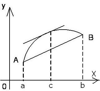
![{\displaystyle f:[a,b]\rightarrow \mathbb {R} ,\;a,b\in \mathbb {R} ,\;a<b}](https://services.fandom.com/mathoid-facade/v1/media/math/render/svg/d3987b334fec4de70bdf0bace6aeea3750c1aca2)
![{\displaystyle [a,b];\!}](https://services.fandom.com/mathoid-facade/v1/media/math/render/svg/edd0ad2080dc8de9fcac4474a234eeba8e2c4664)


![{\displaystyle f:[1,3]\rightarrow \mathbb {R} ,\;f(x)={\begin{cases}x,&daca\;1\leq x\leq 2\\{\frac {x^{4}}{2}}+1,&daca\;2<x\leq 3\end{cases}}\!}](https://services.fandom.com/mathoid-facade/v1/media/math/render/svg/f7ca0433fb2d334b0ab666060eaea3dbd66f89b3)


![{\displaystyle [0,x];\!}](https://services.fandom.com/mathoid-facade/v1/media/math/render/svg/fb37824b65020de1487303c03f13f82fde476ae7)


